
Who doesn’t remember their first love? In my case, in the coding world, my first love was Stata. I clearly remember my first job as a research assistant to Laura Atuesta. Learning Stata implied an important learning curve since this language was used in my university for my classes, my work, and research. I did my bachelor’s thesis with Stata, and, being honest, I just have great memories using Stata because it was the first time that I’ve feel capable of doing multiple things. There my curiosity for data science and coding started. However, like any other Story love (that may be doesn’t end well), I met R. I would say with this language my interest and passion for coding exploded. Since then, I stopped using Stata and fall in love completely for R. Syntaxis, open-source building community and the approach that you can have with this language are just one of the multiple reasons why I decided to keep learning with R. It doesn’t matter what happens, Stata will be always in the bottom of my heart and my first love since it was the first coding language that I learned.
Because of this and because I know that different people and scholars are using Stata and they are curious about what R offers, here is an essential guide of commands for doing some data wrangling, analysis, and running some models. Of course, I don’t cover plenty of things, but this is just to show the differences between using R and Stata. I’m sorry if I don’t use the new Stata approaches since I learned the version 11º or 12º and now the are in the 17º version, however, the commands still can be useful.
We are going to work a lot with the dplyrpackage. You need to load the package just once when you open your environment. If you have any question, please check our other material to start learning R. However, the best way to learn is try different approaches (;
Working directory

/*Working directory path*/
pwd

/*Changes the working directory path*/
cd c:\myfolder\data ![]()

Packages
/*Install package*/
ssc install abc
Once is installed, we don’t need to “load it”
![]()
#Working directory path
install.packages("tidyverse")

#Load library
library(tidyverse)
Help
/*Get help with the command regression*/
help regress
![]()
#Help with mutate function from dplyr package
?mutate()
Load Data
CSV Files
/*Import csv file*/
import delimited "my_data.csv", clear
![]()
library(readr)

#Use read_csv2
df_data <- read_csv2("data.csv")

#Using read.table function with comma separator
df_data <- read.table("my_data.csv",
                      sep = ",",
                      header = TRUE)
Excel Files
/*Import excel file*/
import excel "df_data.xlsx",
sheet("Sheet1") firstrow clear![]()
#With readxl package
library(readxl)
df_data <- read_excel("my_data.xlsx",
                      sheet = "Sheet1")

#With openxlsx package
library(openxlsx)
df_data <- read.xlsx("my_data.xlsx",
                     sheet = "Sheet1")
Stata Files (.dta)
/*Import excel file*/
use "df_data.dta", clear![]()
Explore Data
Remember the difference between R and Stata. While in R you need to specify which object (or data) you want to work with, in Stata, the variables are loaded, so it’s easier to work with them.
/* Provides the structure of the dataset */
describe

/*Basic descriptive statistics */
summarize variable1 variable2

/*Lists the variables in the dataset */
ds

/* First 10 observations */
list in 1/10

/* Last 10 observations */
list in -1/10

/* Show first 10 observations of the */
/*  first three variables of our data */
list var1-var3 in 1/10


/*View data */
browse ![]()
#Provides the structure of our data
str(df_data)

#Basic descriptive statistics
summary(df_data)

#Lists the variables of our data
names(df_data)

#Show first 10 observations of our data
head(df_data, n = 10)

#Show last 10 observations of our data
tail(df_data, n = 10)

#Show first 10 observations of the
# first three variables of our data
df_data[1:10, 1:3]

# With dplyr, this would be other option
library(dplyr)
df_data %>% slice(1:10) %>% select(1:3)

#View data
View(df_data)
Missing Data
/* Provides the structure of the dataset */
missing variable1 variable2 variable3
![]()
Rename variables
/* How to rename */
rename oldname newname

rename lastname lastname2
rename firstname firstname2
rename studentstatus studentstatus2
rename averagescoregrade avgscore
![]()
Label variables
label variable w "Weight"
label variable y "Output"
label variable x1 "Predictor 1"
label variable x2 "Predictor 2"
label variable age "Age"
label variable sex "Gender"![]()
Value labels
/* Value labels for the codes */
label define label1 1 "Option 1"
2 "Option 2" 3 "Option 3" 4 "Option 4"
5 "Option 5"
/* Assign the value labels to the codes */
label values code label1![]()
#Load labelled package
library(labelled)

#Define the value labels for the codes
labels <- c("Option 1", "Option 2",
            "Option 3", "Option 4",
            "Option 5")
df_data$code <- labelled(df_data$code,
                         labels = labels)
#Define the value labels for the codes
labels <- c("Option 1", "Option 2",
"Option 3", "Option 4",
"Option 5")
df_data$code <- factor(df_data$code,
levels = 1:5,
labels = labels)In this approach, you can assign values to numeric or character variables
Group variables
/* Value labels for the codes */
collapse (mean) var1, by(var2, var3)

list var2 var3 var1![]()
Merge two datasets
/* Exact match on the key variable(s). */
use dataset1.dta, clear
merge 1:1 id using dataset2.dta
/* Each observation in the first dataset */
merge 1:m id using dataset2.dta
/* Each observation in the second dataset */
merge m:1 id using dataset2.dta
/* Each observation many-to-many merge */
merge m:1 id using dataset2.dta
Remember that we need to have our data1 in the same path
![]()
#Load dplyr package
library(dplyr)

#1:1 using inner join
df_merged_inner <- inner_join(df_1, df_1,
                              by = "id1")

#1:m using left join
df_merged_left <- left_join(df_1, df_1,
                            by = "id1")

#m:1 using right join
df_merged_right <- right_join(df_1, df_1,
                              by = "id1")

#m:m using full join
df_merged_full <- full_join(df_1, df_1,
                            by = c("id1",
                                   "id2"))
#You can merge with more tha one variable
Create sequence/ids
Drop variables
Frequencies/Tabulation
/* Cross-tabulate 3 variables*/
tabulate var1 var2 var3

/* Cross-tabulate with row and
column percentages */
tabulate var1 var2, row col![]()
Statistics
Summary
Linear Model
/* Fit a linear model */
regress mpg weight length foreign

/* Print summary */
estimates table![]()
Logistic Model
/* Fit a logistic regression model */
logit foreign weight length

/* Print summary */
estimates table![]()
Poisson Model
/* Fit a Poisson regression model */
poisson accidents weight length foreign

/* Print summary */
estimates table![]()
Plots
Scatter plot
/* Create scatter plot */
scatter price mpg![]()
Line plot
/* Create Line plot */
twoway line le_w le_y, xlabel(1950(10)2010)![]()
Bar plot
/* Create a Bar plot */
graph bar (count) rep78, over(foreign)![]()
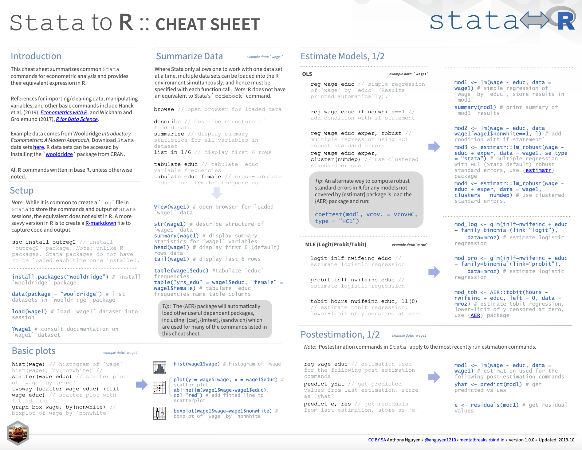
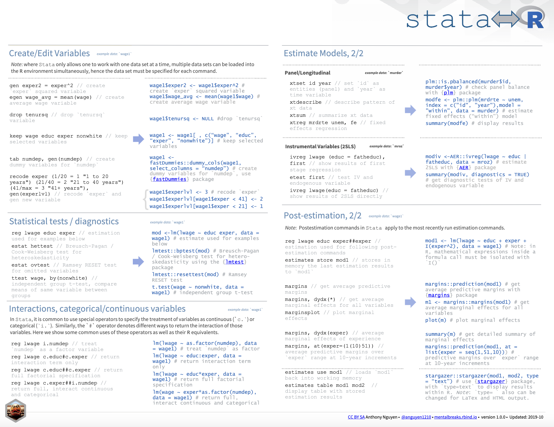
I also want to provide a good cheat sheet that contains more information about the differences between Stata and R.
Cheat Sheet: Stata to R
RStata
Believe it or not, R has a package called RStata. This package Stata interface allows the user to execute Stata commands (both inline and from a .do file) from R. I leave herethe package. Looks interesting; however, I personally prefer to use a language as expected.
Conclusion
In conclusion, the decision to transition from one to the other should be made based on the user’s specific needs and preferences. This notebook shows you the differences between Stata and R. At the end, use the language you prefer, but in my own experience, R was a life changer.
References
Jutkowitz, E., Pizzi, L. T., Shewmaker, P., Alarid‐Escudero, F., Epstein‐Lubow, G., Prioli, K. M., … & Gitlin, L. N. (2023). Cost effectiveness of non‐drug interventions that reduce nursing home admissions for people living with dementia. Alzheimer’s & Dementia.